
Microsoft Excel has just added, since January 13, 2020, a series of revolutionary functions that will greatly simplify the creation of your various management reports as well as your dashboards. The big new feature is the introduction of dynamic matrix functions.
These new functions allow you to create formulas and return multiple results to a range of cells in the worksheet based on a formula entered in a single cell. This behavior is called “buckling” and the results appear within a “buckling range”.
All results are dynamic. When the source content changes, the results are dynamically updated to stay in sync.
Any formulas that return many results will now flow to many cells.
Example:
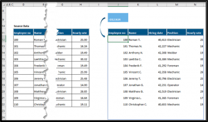
The basic rules are as follows:
- The formula “lives” only in cell J12 (grayed out cell), ie only this cell can be modified.
- To delete the spilled cells, you must delete cell J12.
- Changes to the source data will be reflected in the dumped cells.
- The dynamic range feature is not fully supported between workbooks and workbooks must be opened. Use Power Query instead of referring to other Excel workbooks.
- To refer to a dynamic range, you must use the sign “#”.
- When a cell spills into another cell with content, you will get a new error message #SPILL!.
- To block the discharge of a formula, one must add the following sign: “@” at the beginning of the formula.
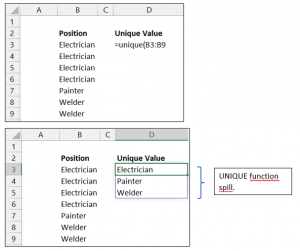
Here is an example with the use of the UNIQUE function:
When you enter the UNIQUE function in cell D3, the result of the function flows into the cells.
Training Excerpt: Excel 365 Dynamic Matrix Functions for Controller and Analyst